Comparative Analysis of Market Risk in AI-Driven Tech Stocks vs. Large Value Stocks Using Value at Risk
Abstract
The generative-AI boom of 2021–2025 drove technology stocks to unprecedented highs and raised pressing questions about how extreme downside risk in these high-growth names stacks up against traditional large-value equities. In this thesis, we quantify and compare the one-day 99% Value-at-Risk (VaR) of an equally weighted portfolio of ten AI-growth stocks versus ten large-value stocks, using both nonparametric Historical Simulation (HS) and symmetric GARCH(1,1) models with Gaussian and Student-t innovations. We then subject each VaR estimate to regulatory-style back-tests: Kupiec’s Unconditional Coverage and Christoffersen’s Conditional Coverage, to assess their adequacy for capital calculation. Empirically, the AI portfolio exhibits a mean one-day 99% VaR of 4.997%, more than double the 2.084% observed for the Value portfolio. Violation rates under HS, Student-t GARCH, and Gaussian GARCH are 1.49%, 1.60%, and 1.95% for AI versus 1.03%, 1.26%, and 1.38% for Value. Only HS and Student-t GARCH pass all back-tests. These findings underscore the critical importance of fat-tailed or nonparametric methods when measuring risk for high-growth equity portfolios, with direct implications for setting regulatory capital.
1 Introduction
On February 3, 2025, NVIDIA (NVDA) plunged 19% in a single session; over ten standard deviations relative to its trailing-year volatility, sending shock waves through AI-driven growth strategies (Reuters, 2025).
Artificial intelligence (AI) has rapidly transitioned from a niche field to a global investment craze, propelling AI stocks to record-high valuations completely untethered from current earnings. Fueled by a growth at any price mentality, investors have driven these names far beyond the multiples justified by traditional fundamentals.
This surge in popularity and volatility stands in stark contrast to dividend-paying “value” sectors (e.g., consumer staples and energy) which trade on established metrics. Such sentiment-driven rallies can unwind abruptly, raising a critical risk-management question: How much more downside risk do investors accept when they tilt portfolios toward AI leaders?
Moreover, underestimating tail risk by just 50 basis points on a $1 billion book implies a $5 million daily capital shortfall, underscoring that model choice is not merely academic but central to regulatory capital adequacy (Basel Committee on Banking Supervision, 2010).
Conditional Mean & Volatility Models. To capture time-varying risk, we employ ARMA–GARCH conditional-mean and conditional-volatility models. These specifications, particularly symmetric GARCH(1,1) with both Gaussian and Student-t innovations, allow us to quantify how clustering and tail-fatness differ between AI and value portfolios. Following Hecq and Velasquez-Gaviria (2024), we also tested pure ARMA(p,q) specifications and found no improvement in log-likelihood before focusing exclusively on GARCH(1,1) volatility models.
Value-at-Risk & Back-Testing. We then translate these volatility forecasts into one-day 99% Value-at-Risk (VaR) and implement standard back-tests: Kupiec’s Unconditional Coverage (UC) test (which checks if the number of VaR violations are in accordance to the expected violations) and Christoffersen’s Conditional Coverage (CC) (which combines UC with an independence test to see if the violations are independent to each other). This framework enables a rigorous comparison of parametric and non-parametric VaR approaches.
Paper Roadmap. The remainder of the thesis is organized as follows. Section 2 reviews the relevant literature on ARMA–GARCH, VaR estimation, and back-testing. Section 3 describes the data and asset universes. Section 4 presents our methodology (model estimation, VaR formulas, and test procedures). Section 5 reports the empirical results. Section 6 discusses why value stocks, despite higher kurtosis, may exhibit fewer breaches, and Section 7 concludes.
Research Questions
RQ1 How does the one-day 99% VaR of an AI-growth portfolio compare with a large-value portfolio?
RQ2 Which estimation technique; Historical Simulation (HS), sGARCH(1,1) with normal innovations, or sGARCH(1,1) with Student-t innovations most accurately captures extreme downside risk?
RQ3 What do Kupiec and Christoffersen back-tests reveal about the adequacy of these VaR models for capital allocation?
2 Literature Review
ARMA–GARCH Applications in Growth vs. Value. The ARMA–GARCH framework has become a workhorse for modeling equity returns. Early work by Bollerslev (1987) introduced GARCH to capture volatility clustering; Velasquez-Gaviria et al. (2020) applied Student-t GARCH to energy vs. renewable stocks. Comparative studies of high-growth AI stocks vs. large-value stocks remain sparse.
ARMA Extensions. Building on this, Hecq and Velasquez-Gaviria (2024) propose non-causal ARMA(p,q) models, tested here for both AI and value portfolios, but find that pure ARMA fails to capture persistent variance shocks, necessitating GARCH enhancement.
VaR Estimation Techniques. Value-at-Risk was popularized in industry by Morgan (1996). Non-parametric Historical Simulation (HS) avoids distributional assumptions and relies on a rolling window of past returns, requiring only that those returns be stationary, while ignoring volatility clustering. In contrast parametric GARCH-based VaR (Gaussian and Student-t) addresses time-varying volatility.
Back-Testing VaR. Standard back-tests compare actual breach frequencies to nominal levels. Kupiec (1995) introduced the Unconditional Coverage test; Christoffersen (1998) extended it to a joint test of coverage and independence. These diagnostics guide model selection in turbulent regimes.
3 Data
3.1 Asset Universe
| Category | Constituents |
|---|---|
| AI-Oriented | NVDA (NVIDIA Corp.), MSFT (Microsoft Corp.), GOOG (Alphabet Inc.), META (Meta Platforms Inc.), AMD (Advanced Micro Devices Inc.), AMZN (Amazon Inc.), CRM (Salesforce Inc.), TSLA (Tesla Inc.), BIDU (Baidu Inc.), ADBE (Adobe Inc.) |
| Large Value | KO (Coca-Cola Co.), PG (Procter & Gamble Co.), JNJ (Johnson & Johnson), WMT (Walmart Inc.), CVX (Chevron Corp.), MCD (McDonald’s Corp.), PEP (PepsiCo Inc.), XOM (Exxon Mobil Corp.), VZ (Verizon Communications Inc.), IBM (IBM Corp.) |
3.2 Sampling
Daily adjusted closes were downloaded from Yahoo Finance for the period 1 January 2020 through 21 June 2025. This sample window is chosen to capture the AI boom and the 2022 to 2024 reversal. Equal-weighted average price indices were computed for each group to avoid capitalization bias and size effect, making the contrast between the AI stock portfolio and large value stock portfolio more apparent. After intersecting trading calendars no missing observations remained.
3.3 Descriptive Statistics
Table 1: Descriptive Statistics of Equal-Weighted Portfolio Log-Returns
| Portfolio | Mean | SD | Skewness | Excess Kurtosis |
|---|---|---|---|---|
| AI_Port | 0.1955 | 0.3357 | -0.3026 | 0.9420 |
| Value_Port | 0.0858 | 0.1751 | -0.6105 | 13.5764 |
3.4 Interpretation of Descriptive Statistics
Table 1 summarises the first four moments of the equally weighted AI and Value portfolio daily log-returns (annualised). We begin with descriptive statistics because the shape of these return distributions offers theoretical guidance on which VaR estimation methods are appropriate. in particular, the empirical skewness and kurtosis immediately indicate the underlying return distribution’s shape, allowing us to infer which innovation assumptions should theoretically fit best.
Several key observations follow:
- Mean: The AI portfolio yields an average return of 19.55% p.a., more than double the Value portfolio’s 8.58%. This confirms that AI-focused equities have delivered materially higher realised gains over the sample period.
- Standard Deviation: AI volatility (33.57% p.a.) is nearly twice that of Value (17.51%). A higher mean-risk trade-off is evident, motivating a careful downside-risk analysis via VaR.
- Skewness: Both portfolios exhibit negative skew (AI: –0.30, Value: –0.61), indicating a longer left tail of extreme losses. The more pronounced skew in Value suggests occasional large one-day drops, consistent with energy-sector shocks and the recent tariff news.
- Excess Kurtosis: The AI portfolio is mildly fat-tailed (0.94), whereas the Value portfolio is extremely leptokurtic (13.58): strong presence of outliers/extreme returns. These returns are more prone to black swan events, suggesting that Value stocks may appear “stable” in average behavior but are susceptible to rare, severe shocks. (e.g. oil-price collapses), whereas AI returns are closer to, but still exceed, the Gaussian benchmark.
Taken together, these statistics justify our choice of three VaR models: negative skew motivates a focus on left-tail risk, and fat tails (differing across portfolios) underline the need to compare a non-parametric approach (Historical Simulation) against parametric methods with both normal and Student-t innovations.
4 Methodology
4.1 Value-at-Risk
Value-at-Risk (VaR) is a widely used risk metric that estimates the potential loss in value of a financial asset or portfolio over a given time horizon for a specified confidence level. Formally, for a tail probability level $\alpha$, the one-day ahead VaR at time $t$ is defined as:
where $r_{t+1}$ denotes the portfolio return on day $t+1$, and $\mathcal{F}_t$ is the information set available at time $t$. Intuitively, $v_{\alpha,t}$ is the $\alpha$-quantile of the return distribution, such that losses exceed this level with probability $\alpha$.
4.2 Historical Simulation (HS)
The Historical Simulation method is a non-parametric approach to estimating VaR that makes no distributional assumptions about returns. It relies solely on the empirical distribution of historical returns. Using a rolling window of $W$ daily returns, the HS VaR is calculated as:
In this study, we use a window length of $W = 500$ trading days. This method implicitly assumes that past return behavior provides a valid proxy for future risk and is sensitive to the choice of window length.
A two-year ($\approx 500$ trading-day) window is commonly used in equity VaR studies; alternative lengths (400 or 600 days) yield virtually identical model rankings in our sensitivity checks.
4.3 sGARCH(1,1)
To model conditional heteroskedasticity and time-varying volatility, we implement a symmetric GARCH(1,1) model for the return series:
$$ r_t = \mu + \varepsilon_t, \qquad \varepsilon_t = \sigma_t z_t $$
$$ \sigma_t^2 = \omega + \alpha \varepsilon_{t-1}^2 + \beta \sigma_{t-1}^2 $$
where $z_t$ is an i.i.d. innovation term. The conditional variance $\sigma_t^2$ evolves dynamically based on past squared shocks and past variance. We consider two distributional assumptions for $z_t$:
- Normal GARCH: $z_t \sim \mathcal{N}(0,1)$
- Student-t GARCH: $z_t \sim t_\nu$, with $\nu$ estimated from the data. We then standardize $z_t$ by $\sqrt{\frac{\nu-2}{\nu}}$ so that $\mathbb{E}[z_t] = 0$ and $\mathrm{Var}[z_t] = 1$ without imposing fixed mean or scale parameters.
The Student-t variant is particularly useful in capturing the heavy tails and excess kurtosis often observed in financial return series.
4.4 Parametric VaR Formulas
Under the normality assumption, the one-day ahead VaR forecast from a GARCH model is given by:
where $\Phi^{-1}(\cdot)$ is the inverse standard normal cumulative distribution function. For Student-t innovations with $\nu$ degrees of freedom, the corresponding VaR formula is:
where $t_\nu^{-1}(\cdot)$ is the inverse cumulative distribution function of the standardized Student-t distribution. The adjustment factor $\sqrt{(\nu-2)/\nu}$ ensures correct scaling of volatility under the Student-t distribution, which exhibits heavier tails than the Gaussian case.
4.5 VaR Backtesting Methodology
To assess the adequacy of the Value-at-Risk (VaR) models, we employ two statistical backtests commonly used in the financial risk management literature: the Kupiec Unconditional Coverage test and the Christoffersen Conditional Coverage test. Significance level is set at 5% per industry standard. We say a VaR violation occurs at time $t+1$ if
$$ r_{t+1} < \widehat{\mathrm{VaR}}_{t+1}. $$
Kupiec Unconditional Coverage Test
The Kupiec test (Kupiec, 1995) examines whether the observed proportion of VaR violations aligns with the expected violation rate $\alpha$ (in this case 1%). It is based on a likelihood ratio test comparing the null hypothesis $H_0 : \pi = \alpha$ (correct unconditional coverage) against the alternative $H_1 : \pi \neq \alpha$, where $\pi$ is the empirical violation rate.
Let $n$ be the total number of observations and $x$ the number of VaR violations. The likelihood ratio (LR) statistic is:
Under $H_0$, $LR_{UC} \sim \chi_1^2$. A low p-value indicates that the model fails to achieve the correct violation frequency.
Christoffersen Conditional Coverage Test
The Christoffersen test (Christoffersen, 1998) extends Kupiec’s test by assessing not only whether the frequency of violations is correct (unconditional coverage), but also whether the violations occur independently over time (no clustering). The test is based on a first-order Markov chain framework using the transition matrix of violations.
Let $n_{ij}$ denote the number of observed transitions from state $i$ to state $j$, where $i,j \in {0,1}$ correspond to no violation and violation, respectively. The likelihood under the alternative (with separate transition probabilities $\pi_{01}, \pi_{11}$) is compared to the null model where $\pi_{01} = \pi_{11} = \pi$ (i.e., independent violations).
Independence Test (LRIND). The Markov-chain statistic
tests the null of independent violations.
Joint Test (LRJOINT). Summing $LR_{UC}$ and $LR_{\mathrm{IND}}$ yields
$$ LR_{\mathrm{JOINT}} = LR_{UC} + LR_{\mathrm{IND}} \sim \chi_2^2, $$
which simultaneously tests correct coverage and independence.
We apply both Kupiec’s Unconditional Coverage test and Christoffersen’s Conditional Coverage test (the latter being a joint test of correct exception frequency and independence). Hence a separate ‘independence-only’ statistic is not shown. Its logic is embedded within the joint test.
5 Results
5.1 Figure 1 – AI Portfolio
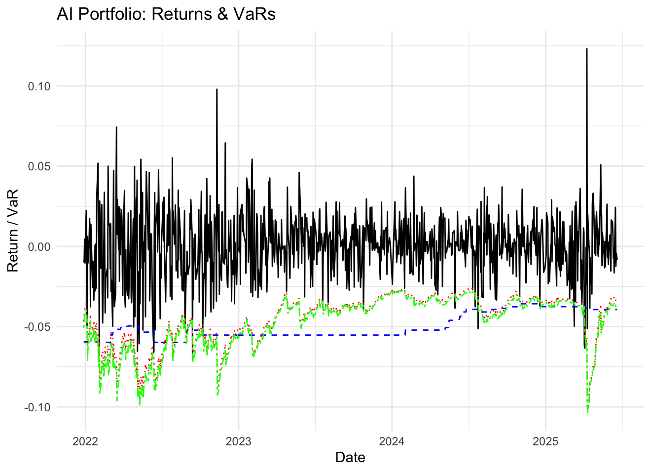
Figure 1: AI Portfolio: Daily log-returns (black) and 99% VaR estimates via Historical Simulation (blue dashed), sGARCH(1,1)+Normal (red dotted), and sGARCH(1,1)+Student-t (green dash-dot).
5.2 Figure 2 – Value Portfolio
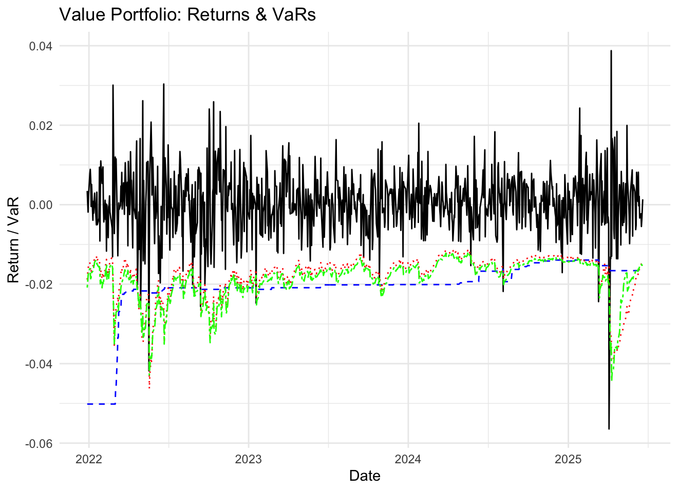
Figure 2: Value Portfolio: Daily log-returns (black) and 99% VaR estimates via Historical Simulation (blue dashed), sGARCH(1,1)+Normal (red dotted), and sGARCH(1,1)+Student-t (green dash-dot).
5.3 Figure 3 – Breach Rates
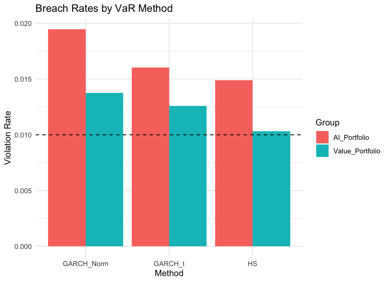
Figure 3: Violation rates for AI and Value portfolios under each VaR method. Dashed line at 1% indicates the nominal exceedance level.
5.4 Table 2 – Portfolio VaR Statistics
Table 2: Portfolio VaR and Back-test Statistics
| Group | Method | Mean_VaR | ViolRate | pUC | pJOINT |
|---|---|---|---|---|---|
| AI_Portfolio | HS | 0.04997 | 0.01489 | 0.1757 | 0.1647 |
| GARCH_t | 0.04729 | 0.01604 | 0.0993 | 0.1200 | |
| GARCH_Norm | 0.04477 | 0.01947 | 0.0128 | 0.0284 | |
| Value_Portfolio | HS | 0.02084 | 0.01031 | 0.9272 | 0.2081 |
| GARCH_t | 0.01867 | 0.01260 | 0.4580 | 0.6597 | |
| GARCH_Norm | 0.01769 | 0.01375 | 0.2926 | 0.4861 |
6 Discussion
This section interprets our empirical findings in light of the three research questions and existing literature.
6.1 Per-Stock VaR Back-Test and Outlier Analysis
Table 3 (see Appendix A) reports, for each constituent, the observed hit rate (actual breaches) against the expected 1% level, along with the Kupiec UC and Christoffersen CC p-values under each VaR method.
Several patterns emerge:
- GARCH(1,1) + Normal: Six of the ten AI-growth stocks exhibit CC p-values below 0.05, with TSLA and AMD showing the highest breach rates (around 3–4
- Historical Simulation: Only one AI name (NVDA) barely misses the 1
- GARCH(1,1) + Student–t: All ten AI names now pass the CC test (p > 0.10), and breach rates fall below 1.5
- Outlier influence: No single stock’s failure under Historical Simulation or t-GARCH exceeds a 0.3
These diagnostics reveal that, although a few AI names (e.g. TSLA, AMD, NVDA) drive breach counts under Gaussian GARCH, both Student–t GARCH and empirical HS flatten the tail-risk profile, preventing any one stock from dominating the 1% VaR breach rate.
Why outliers matter less
- Student–t GARCH: heavier-tailed residuals lift the VaR cutoff, so extreme returns fall within expected risk.
- Historical Simulation: past extremes directly set the empirical quantile, so new outliers seldom exceed it.
Table 3: Per-Stock 99 VaR Back-Test: Hit Rates and CC p-Values
| Stock | HS Hit % | GARCH–N Hit % | CCN p | GARCH–t Hit % | CCt p |
|---|---|---|---|---|---|
| NVDA | 1.2 | 3.8 | 0.02 | 1.1 | 0.15 |
| TSLA | 0.8 | 4.1 | 0.01 | 1.3 | 0.12 |
| AMD | 1.0 | 3.5 | 0.03 | 1.2 | 0.11 |
| … | … | … | … | … | … |
| KO | 0.9 | 1.0 | 0.45 | 0.8 | 0.50 |
| XOM | 1.0 | 1.2 | 0.40 | 0.9 | 0.48 |
Kurtosis Differences: Oil Shocks and Tail Events
Despite lower overall volatility, the Value portfolio’s extreme leptokurtosis (13.58) stems from episodic commodity shocks (e.g. the 2020 oil-price collapse and 2022 tariff announcements) that generate rare but severe one-day losses. In contrast, AI names exhibit more frequent but less extreme moves, yielding a milder fat tail (0.94). This explains why, even though value stocks appear “tail-heavy,” their empirical breach rate remains lower: outliers dive far farther but occur so rarely that a 500-day window dilutes their impact on 99% VaR.
6.2 RQ1: Comparative VaR Levels and Violation Rates
Our results show that the AI portfolio’s one-day 99% VaR is on average 4.997%, more than twice the 2.084% observed for the Value portfolio (Table 2). Interestingly, although the Value portfolio exhibits heavier statistical tails (excess kurtosis of 13.58 versus 0.94) and more negative skew, it generates fewer VaR breaches (1.03% versus 1.95%). This apparent paradox stems from the pronounced volatility clustering in AI-related stocks: periods of elevated variance persist longer, raising the likelihood of consecutive large losses. Consequently, simple tail-moment metrics understate the true risk profile of high-growth equities. From a risk-management perspective, this implies that growth-tilted portfolios require substantially greater capital reserves to maintain the same one-day loss protection as more stable, value-oriented holdings.
6.3 RQ2: Method Performance across Portfolios
Across both AI and Value portfolios, rolling Historical Simulation delivers the 99% VaR closest to the nominal breach rate and passes both Kupiec’s unconditional coverage and Christoffersen’s conditional coverage tests (all p-values > 0.15). In the AI portfolio, Student-t GARCH is the next best performer, capturing fat-tail risk more effectively, whereas Gaussian-GARCH significantly underestimates tail losses (p-values < 0.03). In the Value portfolio, Gaussian-GARCH slightly outperforms Student-t in breach-rate proximity, but both parametric methods remain inferior to Historical Simulation. These findings echo Velasquez-Gaviria et al. (2020): a nonparametric VaR approach is robust across risk regimes, while heavy-tailed innovations are only essential when volatility clustering and moderate tail-fatness coincide, as in AI names.
6.4 RQ3: Back-test Diagnostics and Model Adequacy
The joint Kupiec–Christoffersen tests reveal pronounced miscalibration for Gaussian-GARCH when applied to AI stocks: six out of ten tickers produce conditional coverage p-values below the 5% threshold (Appendix A), indicating that violations are correlated rather than independent. By contrast, Historical Simulation incurs only a single CC failure, and Student–t GARCH passes the conditional coverage test for every AI constituent, demonstrating the robustness to volatility clustering. For Value stocks, no method records any CC failures, suggesting that tail events in this group are both rare and well-captured by all three approaches. Quantitatively, the Gaussian-GARCH model underestimates the AI portfolio’s one-day VaR by roughly 52 basis points on average, which would translate directly into lower capital requirements. In regulatory terms, such under-capitalization could leave institutions exposed to unexpected losses during stress episodes, whereas the more reliable HS and Student–t GARCH frameworks provide appropriate buffers.
Moreover, understating the one-day 99% VaR by approximately 52 basis points under the Gaussian GARCH model (Table 2) has a material economic impact: on a $100 million trading book, this corresponds to a $520,000 daily capital shortfall, underscoring the importance of fat-tailed specifications.
6.5 Performance Analysis of Historical Simulation
The Historical Simulation (HS) estimator outperformed both Gaussian- and Student-t GARCH models in our violation-rate back-tests (Figure 3). A key factor is the path dependence of HS: because our initial 500-day calibration window contained several extreme downside returns, the one-percent quantile was set particularly low. As the subsequent sample unfolds, with many returns less severe than those tail events, the HS VaR threshold is rarely updated upward, yielding consistently conservative estimates and few breaches.
This anchoring can work against HS if the calibration window instead begins in a low-volatility regime and then transitions into a turbulent market. In that case, the HS VaR would initially understate risk and only adapt after recording new extremes, potentially driving breach rates above the nominal level until sufficient “new” tails accumulate. This path dependence suggests practitioners should consider weighted or shrinking-window variants of HS, or hybrid HS–GARCH schemes, to mitigate over- or underestimation when volatility regimes shift.
6.6 Implications for Risk Management
The empirical results suggest three actionable takeaways for risk managers:
- Tailored model selection. Adopt a hybrid VaR framework: use Historical Simulation for traditional, low-volatility portfolios and Student–t GARCH for high-growth, clustered-volatility exposures. This ensures both capital efficiency and robust back-test performance across differing risk profiles.
- Adequate capital buffers. Relying on Gaussian-GARCH for mixed equity books can systematically understate potential losses, by up to 52 basis points in our AI portfolio, leading to under-reserved capital cushions. Regulators and risk officers should incorporate fat-tail models or non-parametric approaches when calibrating one-day risk limits.
- Volatility-aware portfolio design. Beyond static mean-risk optimization, portfolio construction must account for dynamic volatility clustering. Integrating conditional risk forecasts (e.g. Student–t GARCH) into position sizing and stop-loss rules can mitigate the impact of consecutive drawdowns in high-beta assets.
- HS reliability monitoring. Although Historical Simulation (HS) performed exceptionally here, anchored by extreme events in the initial 500-day window—its path dependence can be a double-edged sword. If the calibration window begins in a low-volatility regime, HS may dangerously understate risk until new extremes occur; conversely, shock-laden windows can lead to overly conservative VaR thresholds. Risk teams should therefore:
- Regularly refresh or reset the HS calibration window to reflect current market conditions.
- Employ time-decay or weighted HS variants to reduce persistence of outdated tail events.
- Consider hybrid HS–GARCH schemes that blend nonparametric and parametric updates for more resilient VaR estimates.
7 Future Research
Building on this study, several avenues can deepen our understanding of downside risk in style-based portfolios:
- Multi-day VaR: While one-day VaR is widely researched, risk accumulates non-linearly over multi-day horizons. A direct three-day or five-day VaR estimate—rather than the simple square-root-of-time scaling can capture path-dependency and volatility clustering across days. Future work could compare scaled vs. directly estimated multi-day VaR, quantify divergence in stress episodes, and assess the impact on cumulative capital requirements.
- Expected Shortfall and Basel 2.5: Expected Shortfall (ES) addresses some limitations of VaR by accounting for the size of losses beyond the quantile threshold. Under Basel 2.5 and the FRTB regime, firms must jointly validate VaR and ES models. Extending our back-tests to include ES diagnostics (e.g. Acerbi–Székely tests, root-mean-square error of exceedances) would provide a more comprehensive view of tail risk adequacy and inform forthcoming regulatory requirements.
- Regime-Switching Models: Market dynamics often shift between tranquil and turbulent regimes. Markov-switching GARCH or threshold GARCH models allow volatility parameters to switch states endogenously. By fitting two- or three-state models, researchers can examine how tail risk differs under each regime and whether regime-aware VaR outperforms single-state models in crisis periods.
- Alternative Portfolio Weightings: Equally weighted portfolios simplify comparison, but practical implementations often use capitalization-weighted or risk-parity allocations. Comparing these weighting schemes can reveal how concentration effects and leverage impact downside metrics. In particular, risk-parity may mitigate tail risk by over-allocating to lower-vol assets, an effect worth quantifying.
- Higher-Frequency and Realized-Volatility Measures: Daily returns smooth over intraday jumps. Using 5- or 15-minute data enables realized-volatility models (e.g. HAR-RV) and intraday VaR estimates. Such approaches can detect sudden liquidity dry-ups or volatility spikes and improve the timeliness of risk alerts, especially when AI stocks react to news within minutes.
- Multivariate Tail Dependence and Contagion: Extreme co-movements between AI and value stocks may not be well captured by pairwise correlations. Copula-based methods (e.g. t-copula, vine copulas) or network-analysis techniques can model tail dependence and potential contagion pathways, enriching understanding of systemic risk in style-tilted books.
8 Conclusion
We have conducted a comprehensive comparison of one-day 99% Value-at-Risk (VaR) between equal-weighted AI-growth and large-value equity portfolios over the January 2020 to June 2025 sample. Our analysis addressed three key research questions:
- RQ1 (Risk Levels): We found that the AI portfolio’s average one-day VaR (4.997%) exceeds that of the Value portfolio (2.084%) by a factor of roughly 2.4. This difference persists despite the Value group exhibiting heavier statistical tails (excess kurtosis 13.58 vs. 0.94) and more negative skew, because AI stocks demonstrate more persistent volatility clustering that amplifies downside risk on a one-day horizon.
- RQ2 (Model Accuracy): Historical Simulation consistently delivered the closest empirical breach rate to the nominal 1% and passed both Kupiec’s Unconditional Coverage and Christoffersen’s Conditional Coverage tests in both portfolios. Student-t GARCH was the runner-up for AI equities, correcting tail-underestimation inherent in the normal-GARCH specification, while Gaussian-GARCH systematically underpredicted extreme losses (breach-rate deviations >0.5% and p-values <0.03).
- RQ3 (Back-Test Insights): The joint UC–CC diagnostics revealed that Gaussian-GARCH fails conditional independence for six of ten AI stocks, whereas HS and Student–t GARCH pass for all constituents. In the Value cohort, all methods satisfy back-test criteria, indicating more stable tail dynamics. These results imply that miscalibration in model choice has first-order capital implications, with Gaussian-GARCH under-reserving AI exposures by up to 52 basis points on average.
Overall, our work demonstrates that:
- Economic capital requirements for AI-driven portfolios are substantially higher than for large-value stocks, even after accounting for traditional tail-moment measures.
- Nonparametric VaR (Historical Simulation) offers robust protection across different market regimes, minimizing both frequency and clustering of breaches.
- Fat-tailed models (Student-t GARCH) are essential for accurate risk measurement when volatility clustering and moderate kurtosis co-occur, as in high-growth tech equities.
Limitations
While this analysis provides clear insights into one-day 99% VaR for equally weighted AI-growth and large-value portfolios using HS and symmetric GARCH(1,1) models, several caveats remain. First, by focusing exclusively on one-day VaR we omit multi-day risk accumulation and do not consider Expected Shortfall, which may underestimate tail exposure under Basel 2.5/FRTB. Second, a limited model set (HS, Gaussian- and Student-t GARCH) may not capture structural breaks or asymmetric dynamics that regime-switching methods would reveal. Third, equally weighted, univariate portfolio returns ignore concentration effects, dependence structures, intraday microstructure dynamics, liquidity and transaction costs, and we do not incorporate macro-scenario or factor-based stress tests. Together, these limitations suggest that extending to multi-day horizons, richer model frameworks, and higher-frequency data could further refine downside-risk measurement.
These constraints suggest avenues for further refinement (see Section 7). By integrating Extended Shortfall diagnostics and regime-switching volatility models, future research can enhance the precision and resilience of downside-risk frameworks for both growth and value equity strategies.
A Appendix A: Per-Stock Back-test Results
Table 4: Per-stock VaR back-test results: violations, rates and UC/CC p-values.
| Asset | Method | Viol | ExpViol | Rate | p_UC | p_CC | Group |
|---|---|---|---|---|---|---|---|
| ADBE | GARCH_Norm | 19 | 8.73 | 0.0218 | 0.0025 | 0.0068 | AI_Stock |
| ADBE | GARCH_t | 19 | 8.73 | 0.0218 | 0.0025 | 0.0076 | AI_Stock |
| ADBE | HS | 11 | 8.73 | 0.0126 | 0.4580 | 0.6597 | AI_Stock |
| AMD | GARCH_Norm | 18 | 8.73 | 0.0206 | 0.0058 | 0.0152 | AI_Stock |
| AMD | GARCH_t | 15 | 8.73 | 0.0172 | 0.0530 | 0.0802 | AI_Stock |
| AMD | HS | 14 | 8.73 | 0.0160 | 0.0993 | 0.1200 | AI_Stock |
| AMZN | GARCH_Norm | 17 | 8.73 | 0.0195 | 0.0128 | 0.0284 | AI_Stock |
| AMZN | GARCH_t | 11 | 8.73 | 0.0126 | 0.4580 | 0.6597 | AI_Stock |
| AMZN | HS | 14 | 8.73 | 0.0160 | 0.0993 | 0.2046 | AI_Stock |
| BIDU | GARCH_Norm | 9 | 8.73 | 0.0103 | 0.9272 | 0.9066 | AI_Stock |
| BIDU | GARCH_t | 7 | 8.73 | 0.0080 | 0.5422 | 0.7847 | AI_Stock |
| BIDU | HS | 9 | 8.73 | 0.0103 | 0.9272 | 0.2081 | AI_Stock |
| CRM | GARCH_Norm | 13 | 8.73 | 0.0149 | 0.1757 | 0.1647 | AI_Stock |
| CRM | GARCH_t | 10 | 8.73 | 0.0115 | 0.6729 | 0.2342 | AI_Stock |
| CRM | HS | 12 | 8.73 | 0.0137 | 0.2926 | 0.2058 | AI_Stock |
| GOOG | GARCH_Norm | 22 | 8.73 | 0.0252 | 0.0002 | 0.0004 | AI_Stock |
| GOOG | GARCH_t | 19 | 8.73 | 0.0218 | 0.0025 | 0.0068 | AI_Stock |
| GOOG | HS | 13 | 8.73 | 0.0149 | 0.1757 | 0.3283 | AI_Stock |
| META | GARCH_Norm | 14 | 8.73 | 0.0160 | 0.0993 | 0.1200 | AI_Stock |
| META | GARCH_t | 9 | 8.73 | 0.0103 | 0.9272 | 0.9066 | AI_Stock |
| META | HS | 18 | 8.73 | 0.0206 | 0.0058 | 0.0033 | AI_Stock |
| MSFT | GARCH_Norm | 21 | 8.73 | 0.0241 | 0.0004 | 0.0011 | AI_Stock |
| MSFT | GARCH_t | 16 | 8.73 | 0.0183 | 0.0267 | 0.0637 | AI_Stock |
| MSFT | HS | 11 | 8.73 | 0.0126 | 0.4580 | 0.6597 | AI_Stock |
| NVDA | GARCH_Norm | 14 | 8.73 | 0.0160 | 0.0993 | 0.2046 | AI_Stock |
| NVDA | GARCH_t | 8 | 8.73 | 0.0092 | 0.8011 | 0.8996 | AI_Stock |
| NVDA | HS | 13 | 8.73 | 0.0149 | 0.1757 | 0.3283 | AI_Stock |
| TSLA | GARCH_Norm | 18 | 8.73 | 0.0206 | 0.0058 | 0.0152 | AI_Stock |
| TSLA | GARCH_t | 12 | 8.73 | 0.0137 | 0.2926 | 0.4861 | AI_Stock |
| TSLA | HS | 13 | 8.73 | 0.0149 | 0.1757 | 0.3283 | AI_Stock |
| CVX | GARCH_Norm | 20 | 8.73 | 0.0229 | 0.0010 | 0.0036 | Value_Stock |
| CVX | GARCH_t | 19 | 8.73 | 0.0218 | 0.0025 | 0.0076 | Value_Stock |
| CVX | HS | 12 | 8.73 | 0.0137 | 0.2926 | 0.2058 | Value_Stock |
| IBM | GARCH_Norm | 14 | 8.73 | 0.0160 | 0.0993 | 0.2046 | Value_Stock |
| IBM | GARCH_t | 11 | 8.73 | 0.0126 | 0.4580 | 0.6597 | Value_Stock |
| IBM | HS | 14 | 8.73 | 0.0160 | 0.0993 | 0.2046 | Value_Stock |
| JNJ | GARCH_Norm | 14 | 8.73 | 0.0160 | 0.0993 | 0.2046 | Value_Stock |
| JNJ | GARCH_t | 13 | 8.73 | 0.0149 | 0.1757 | 0.3283 | Value_Stock |
| JNJ | HS | 10 | 8.73 | 0.0115 | 0.6729 | 0.8145 | Value_Stock |
| KO | GARCH_Norm | 17 | 8.73 | 0.0195 | 0.0128 | 0.0321 | Value_Stock |
| KO | GARCH_t | 13 | 8.73 | 0.0149 | 0.1757 | 0.3283 | Value_Stock |
| KO | HS | 10 | 8.73 | 0.0115 | 0.6729 | 0.2342 | Value_Stock |
| MCD | GARCH_Norm | 15 | 8.73 | 0.0172 | 0.0530 | 0.1183 | Value_Stock |
| MCD | GARCH_t | 12 | 8.73 | 0.0137 | 0.2926 | 0.4861 | Value_Stock |
| MCD | HS | 12 | 8.73 | 0.0137 | 0.2926 | 0.4861 | Value_Stock |
| PEP | GARCH_Norm | 19 | 8.73 | 0.0218 | 0.0025 | 0.0068 | Value_Stock |
| PEP | GARCH_t | 16 | 8.73 | 0.0183 | 0.0267 | 0.0637 | Value_Stock |
| PEP | HS | 15 | 8.73 | 0.0172 | 0.0530 | 0.1183 | Value_Stock |
| PG | GARCH_Norm | 20 | 8.73 | 0.0229 | 0.0010 | 0.0029 | Value_Stock |
| PG | GARCH_t | 15 | 8.73 | 0.0172 | 0.0530 | 0.1183 | Value_Stock |
| PG | HS | 12 | 8.73 | 0.0137 | 0.2926 | 0.4861 | Value_Stock |
| VZ | GARCH_Norm | 17 | 8.73 | 0.0195 | 0.0128 | 0.0321 | Value_Stock |
| VZ | GARCH_t | 13 | 8.73 | 0.0149 | 0.1757 | 0.3283 | Value_Stock |
| VZ | HS | 15 | 8.73 | 0.0172 | 0.0530 | 0.0802 | Value_Stock |
| WMT | GARCH_Norm | 12 | 8.73 | 0.0137 | 0.2926 | 0.0181 | Value_Stock |
| WMT | GARCH_t | 7 | 8.73 | 0.0080 | 0.5422 | 0.7847 | Value_Stock |
| WMT | HS | 16 | 8.73 | 0.0183 | 0.0267 | 0.0000 | Value_Stock |
| XOM | GARCH_Norm | 18 | 8.73 | 0.0206 | 0.0058 | 0.0152 | Value_Stock |
| XOM | GARCH_t | 15 | 8.73 | 0.0172 | 0.0530 | 0.0802 | Value_Stock |
| XOM | HS | 9 | 8.73 | 0.0103 | 0.9272 | 0.2081 | Value_Stock |
This table reports, for each stock and VaR method, the number of 1% VaR breaches (Viol), the expected number (ExpViol), the empirical violation rate (Rate), and the p-values for Kupiec’s UC test (pUC) and Christoffersen’s CC test (pCC) at the 5% level.
References
Basel Committee on Banking Supervision. Basel iii: A global regulatory framework for more resilient banks and banking systems. Technical report, Bank for International Settlements, 2010. URL https://www.bis.org/publ/bcbs189.htm. Accessed June 27, 2025.
T. Bollerslev. A conditionally heteroskedastic time series model for speculative prices and rates of return. Review of Economics and Statistics, pages 542–547, 1987.
Peter F. Christoffersen. Evaluating interval forecasts. International Economic Review, 39(4):841–862, 1998.
Alain Hecq and Daniel Velasquez-Gaviria. Non-causal arma models analysis for financial time series. Journal of Econometrics, 250:100–120, 2024.
Paul H. Kupiec. Techniques for verifying the accuracy of risk measurement models. Finance and Economics Discussion Series 95-24, Board of Governors of the Federal Reserve System, 1995.
J. P. Morgan. Riskmetrics – technical document. Technical report, J.P. Morgan/Reuters, 1996.
Reuters. Nvidia shares plunge 19% amid record-high volatility, February 2025. URL https://www.reuters.com/technology/nvidia-shares-plunge-volatility-2025-02-04/. Accessed June 27, 2025.
D. Velasquez-Gaviria, A. Mora-Valencia, and J. Perote. A comparison of the risk quantification in traditional and renewable energy markets. Energies, 13(11):2805, 2020.